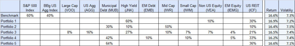
You are pitched multiple ‘tailored’ portfolios that have seemingly very similar risk-return expectations. Beyond the regulatorily mandated disclosures, the distributors/allocators generally point to the historical performance of the portfolios and forecasted performance under scenarios. In Table 1 we take an example of five portfolios with near identical first order risk-return profiles – how would you select?
The baseline financial analysis of the portfolios relies on two baseline facets[1]: (a) the performance measures being considered, and (b) the assumptions embedded in the simulations. Where,
1. Performance measures – there are 100s, varying from simpler ones to those requiring higher order financial engineering. Which ones do you present/understand (especially without losing your audience)? Where, using simplistic or uni-dimensional measures has the risk of accentuating underlying biases and/or instilling unwarranted comfort while not being complete (e.g., using only VaR based, proxy based on a pre-designated asset mix, only stress based, etc.).
2. Simulations have model, market and other assumptions. As opposed to running endless scenarios, most distributors/allocators rely on a few boxed cases from third-party providers (as in the runs, assumptions, regimes, etc.).
Looking at all this can also be overwhelming and/or inconsistently done. So we asked, why can’t there be a way to assess/communicate all the embedded nuances of the portfolios in a simpler, unified way that bridges the financial engineering/jargon? In this Insights piece, we present the advantages of Explainability Index (EI) and Risk of Target (RoT) as the unifying framework of all performance measures (historic or simulated) for consistent portfolio evaluation with simple/explainable visuals. Think of it as a doctor’s report with the thermometer/temperature being the first order of assessment, followed by a set of category indicators of vitals. So, are you worse off than the target (as in have high temperature) and why (as in which performance measures are indicating deviations and can it be fixed)?
Refer to our technical paper[2] – Hirsa, Ding, Malhotra (2023) for the financial engineering and implementation details.
Data
Indices and ETF based model portfolios that have an objective of outperforming the (60% SP500 TR US +40% US Agg Bond TR USD) blend as the benchmark. As illustrated in Table 1, while the security compositions of the portfolios are different, the historic risk-return profiles[3] are quite similar (as a first-order objective function), where at first glance all five can be considered to be viable alternatives. Insights are extendable to all types of portfolios.
We assess the portfolios using traditional analysis and then supplement the assessments with the EI&RoT framework to add color.
Traditional Analysis
This would include assessing (a) Performance Measures, and (b) Simulations.
Performance Measures
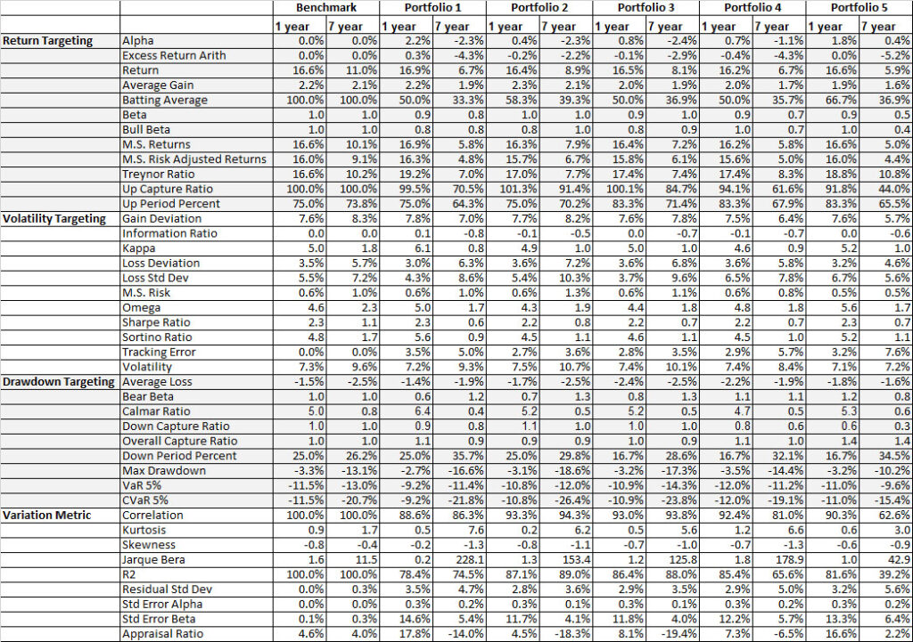
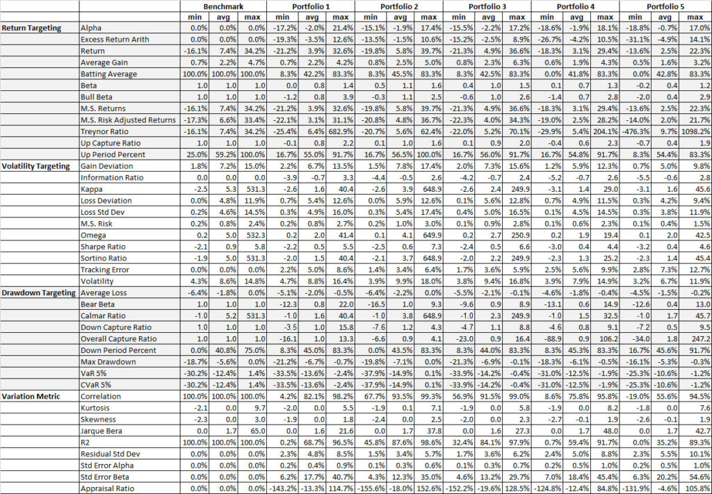
Assessments are based on one or a combination of performance measures. In Table 2, we estimate the 1-year and the 7-year (annualized) measures[4].
Simulations
Figure 1 are the results of a Monte Carlo simulation on the portfolios, where we assume:
- 500 simulated paths
- No regimes in the market
- Returns are normally distributed for all assets, simulated on a monthly frequency
- Return and Volatility are the 7-year historical values evaluate on 2022-12-31
- Correlation is taken from the 7-year monthly return of the assets evaluate on 2022-12-31
- Simulation for a 1 year holding period
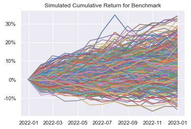
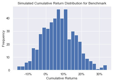

Table 3 gives the simulation results for performance measures of the benchmark and the five portfolios.
For the simulations, beyond the assumptions noted above for the run, some other considerations and assessments could include,
- Regimes with transition probabilities, starting regimes (on/off risk), etc.
- Distributions other than normal e.g., Log-Normal, Gamma, Uniform, Stochastic Process, GAN (VanillaGAN, RegGAN, TaGAN, etc.
- Assumption/stresses – Correlations (over time), Drawdown frequency, Regimes, etc.
Furthermore, in addition to the Traditional analysis, the distributors/allocators may also point to value-add via,
- doing a more fundamental analysis of the assets in the portfolio (in terms of physical due diligence of offering/manager)
- having opinions on the direction of the market
- risk/compliance considerations around existing holdings in the form of concentrations, restrictions, etc.
For this Insights piece, we assume all above one off considerations to be pari-passu, where in the end, we have data and more data from the analysis and the selection will be based on some combination of the aforementioned measures/analysis. Depending on the audience this can be complicated as the discussion becomes a balancing act between level of financial engineering/jargon and explainability.
Take the next step and add color: Explainability Index (EI) and Risk of Target (RoT)
In this piece, we demonstrate a mathematically[5] sound method of supplementing your traditional analysis by (a) estimating the Explainability Index of the portfolio and benchmark (as the Target), and then (b) estimating the Risk of Target (which is an easy way to assess the risk of not meeting the objective function as defined by the Target). Since adding color is a next step to the analysis already done it is not replacing, but supplementing the existing assessment and presentation of your preferred performance measures (historic or simulated). For example, assume you only look at three measures e.g., historic Excess Return, Sharpe and VaR – here the EI calculation simply combines the three as the Index for the portfolios and the related benchmark, and then as a comparative you have the RoT of the portfolios.
Background
We first illustrate the simple and explainable power of the EI&RoT framework with an example of an index and its investable ETF counterpart. Illustration 1 has S&P 500 as the Index (represented by the black circle) and Vanguard S&P 500 ETF (VOO) as the investible parallel (represented by the second circle). RoT[6] adds color (from the EI of the asset versus the target) to the traditional Efficient Frontier plots, where here the RoT of 0% is highlighted in yellow. This means the ETF counterpart is effectively tracking the Index on all measures.
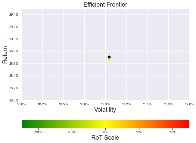
Illustration 2 gives the EI&RoT framework for the same (Index and investible counterpart) and as can be expected the categories are overlapping.
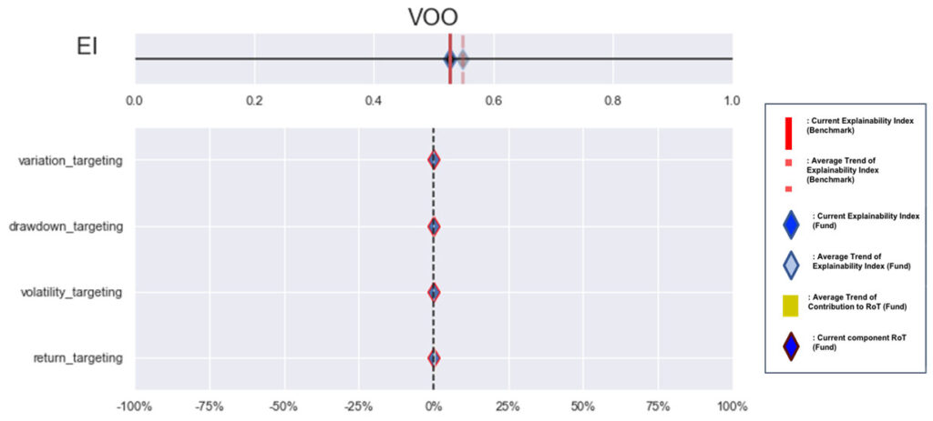
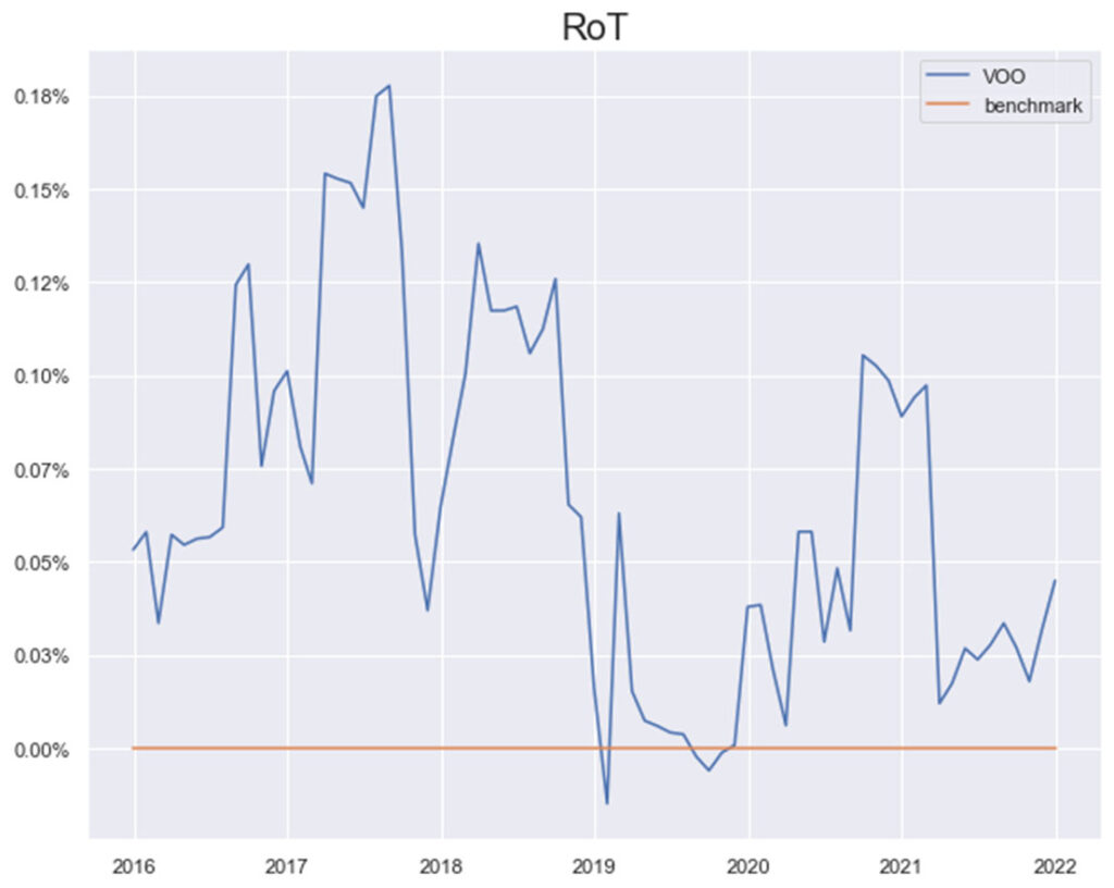
Illustration 3, highlights the RoT over time and we note a marginal difference of <0.18% between the S&P 500 and Vanguard S&P 500 ETF (VOO) as its investible counterpart. This marginal difference can be expected because of fees and other investable aspects. Case in point to select the Index trackers with minimum RoT!
Supplementing Traditional Analysis
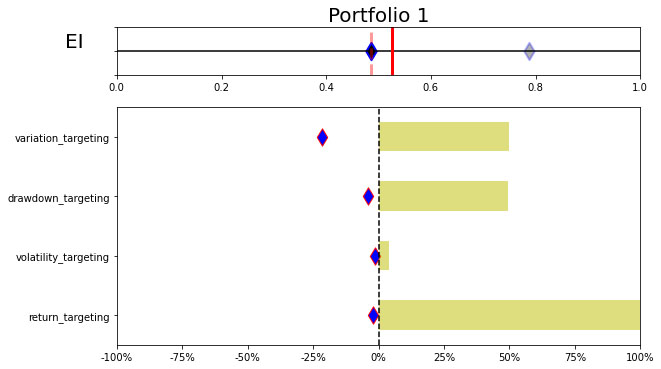
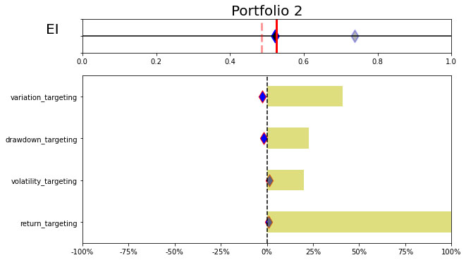
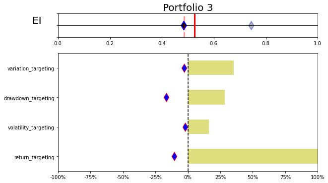
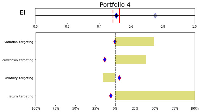
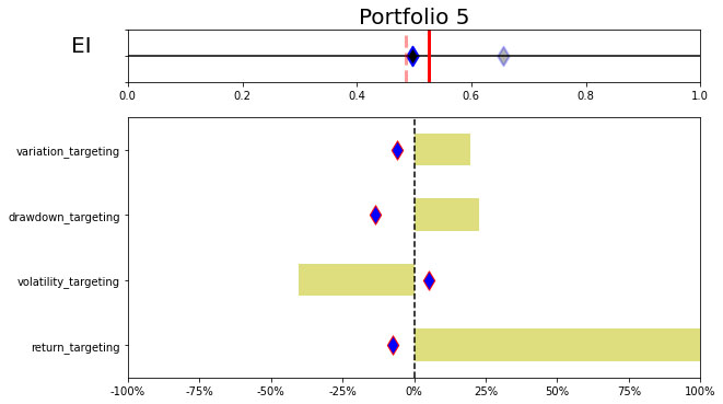
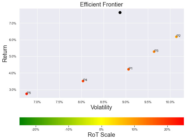
We revert to the portfolio in Table 1 and the performance measures in Table 2. Figure 4 gives near overlapping Efficient Frontier plots showing marginal differentiation as can be expected from the first order measures from Table 1. However, looking at the RoT colors within Figure 4 and as illustrated in Figure 5, Explainability Index (EI) and RoT framework’s granular assessment of each performance measure’s behavior of the five portfolios paints a very different picture.
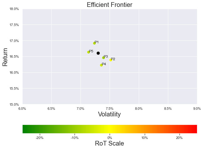

The nuanced assessment of each portfolio’s performance measures versus the Targeted objective function create a level playing field. The multidimensionality capture with simple and explainable visuals should allow the selector to easily evaluate and communicate the RoT in each portfolio.
Illustrations 6 and 7 are Efficient Frontier RoT and EI&RoT frameworks[7] for simulation results in Table 3.
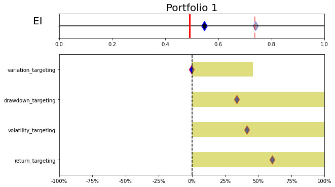
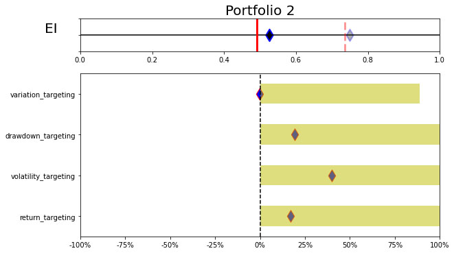
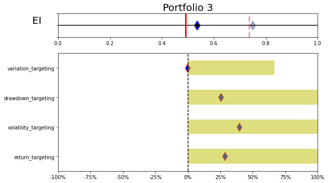
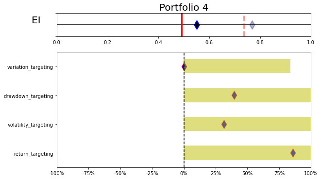
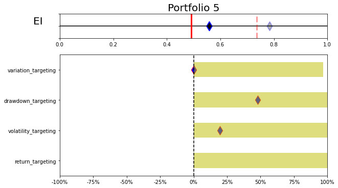
A picture is worth a thousand words or in this case, the picture is worth all financial performance measures! The EI&RoT framework gives an easy visual to note the drivers of divergence from the target benchmark. As such, the EI&RoT framework acts as a control panel to base the objective function and resultant assessment. The amplification of nuances within the uniform presentation of complex and simpler measures should facilitate a better suitability selection choice across the portfolios. So, the question becomes, what aspect of the risk-return profile is important for you to manage? Overall, since EI is directional the lower the EI the better, however it all depends on the objective functions (as defined by the target benchmark here). Once you set the objective function via the weights for the categories then the portfolio with the lowest RoT versus the objective function should be the more suitable choice.
Methodology Comparison
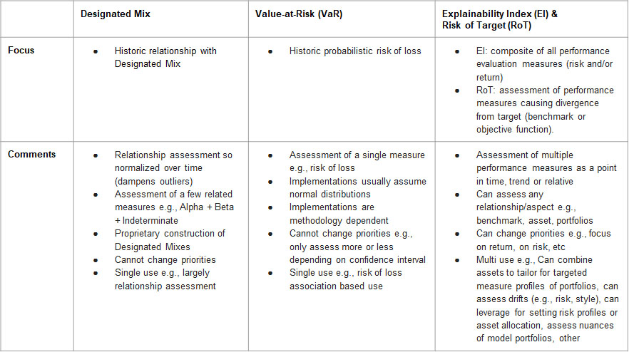
As noted in Table 4, the multi-dimensionality effect captured by the Explainability Index (EI) and Risk of Target (RoT) allows for supplemental control as opposed to a single measure like Value-at-Risk (VaR) or relating portfolios to designated mixes (which are two of the popular methods supported by Software/Solution providers[8]). In Table 4 we did not include the stress testing, concentration and other such risk assessments as those are supplemental and not necessarily used for risk profiling, where the results of such measures can also be inputs for the EI&RoT assessment.
Time to upgrade the baseline VaR analysis, where the application of the EI&RoT framework can be very effective across the Investment Life Cycle including for Asset Selection, Asset Allocation, Portfolio Construction, Risk Management, Asset Planning, etc. The EI&RoT framework’s applicability herein has to account for non-linearity and we will delve into each of these lifecycle components in the subsequent Insights pieces.
Insights 2.10. Mutual Fund Manager Selection – Basic Historic Analysis: Are you always wrong?
We begin by holistically looking at the US mutual fund manager landscape from a historical fund price perspective and assess the ability of widely used performance measures for manager selection. This is done both at the market and individual fund level. Then as simple extensions we evaluate regressions for generally fixed weighting schemes of performance measures over fixed time periods and during discrete regimes. We look at simple back testing and predefined simulations. We will give Insights for every Asset Class.
Insights 2.20. Mutual Funds – Is there value in leveraging larger datasets?
We incorporate larger volumes of macro data, market data, performance measures, holding data, alternative data, etc. We introduce forms of feature engineering to generate signals for regimes, factors, indicators and measures using both raw and reduced datasets. We also introduce synthetic data generation to supplement sparse datasets.
Insights 2.30. Mutual Funds – Machine and Deep learning edge?
We incorporate evolving market conditions, performance measures, weights, events, predictions, etc. by leveraging Machine Learning techniques for real time and simulated multivariate analysis. Then we allow the system to do feature and event engineering by assessing various Deep Learning methods.
Extensions can be drawn to other types of managers, assets and markets. Here we will stay at the framework level, but will refer to our other papers that delve into the technical nuances and discoveries. Additionally, we will share similar series of Machine and Deep Learning framework papers for other aspects of the Investment lifecycle – asset allocation, portfolio management, risk management, asset planning, product development, etc.
These are all underpinnings of the ASK Platform, where it is built to support any/all permutation/combination of data/models/visuals – both traditional and proprietary (via a AI lens).
Email: info@ask2.ai for questions.
NEXT
Insights 2.02. Asset Allocation – Profiles RoTten?
[1] We assume that the other elements of Risk Management, Compliance and other suitability concerns/restrictions (which should be largely standardized processes) have been processed.
[2] Hirsa, Ali and Ding, Rui and Malhotra, Satyan, Explainability Index (EI): Unifying Framework of Performance Measures and Risk of Target (RoT): Variability from Target EI (January 23, 2023). Available at SSRN: https://ssrn.com/abstract=4335455
[3] Evaluation period: 2014-12-31 to 2021-12-31
[4] Estimates are based on monthly returns so impact certain calculations (e.g., CVaR assumed to be VaR for the 1-year period).
[5] In our paper (Hirsa, Ding, Malhotra (2023), we combine many previous works on asset or portfolio performance evaluation measures and propose a unifying framework that captures the various facets of performance evaluation. We transform all the measures to have bounded values between 0 and 1 and use a weighted distance combination to generate a single number that we call an Explainability Index (EI), which itself is in between 0 and 1. This Index is easy to interpret and gives an explicit evaluation of performance by bringing in all measures as manifolds, without losing information. We propose several extensions to this framework, including various categorization or weighting mechanisms on input measures to reflect investor risk preferences, methods to incorporate the variation of measures over time, a geometric summed version which we call Explainability Index, as well as incorporating distributional shifts within Explainability Index. We have also suggested alternative tuning of the score transformation method in the calculation procedure to balance different classes of measures and to generate scaled Index values. We have also extended this approach by computing a relative score that we call the Risk of Target (RoT) which is the comparative Explainability Index of each asset, portfolio, or benchmark. The proposed RoT can be used to rank assets or portfolios, assess composite or component deviations, evaluate point-in-time, relative, or trends, and is helpful in optimization decisions across the Investment Life-cycle. We believe that it is also an effective tool for explaining complex financial engineering and jargon for potentially wider audience engagement.
[6] The current is based on the 1-year and the average is based on 7-year annualized. Analysis assumptions: Measures: Absolute. Time Variation: No. Threshold/Scale: Market Index. Categories: Yes. Weights: Equal. Type: Arithmetic.
[7] The current is based on the 1-year simulated results and the bar is the max of the simulation (similarly can look at average, range, etc). Analysis assumptions: Measures: Absolute. Time Variation: No. Threshold/Scale: Market Index. Categories: Yes. Weights: Equal. Type: Arithmetic.
[8] Detailed assessment versus all solution providers and methods is available upon request.